By Nirek Dandanayak

“This is first in the series of outstanding Economics ILAs written by RGS students this year, which we plan to publish on the 1509 to recognise their efforts and ensure their work reaches a wider audience.” – Mr Stratford, Head Of Economics

Introduction:
According to traditional economic theory, competition should always lead to higher quantity and
quality of output. When producers are faced with competition in the market, they are forced to
decrease prices and produce a higher quantity and quality of goods in order to stay competitive and
stay in business. In the context of sports, this would mean that when the competition between players
is more intense, their performance should improve. However, the superstar effect explains a different
outcome. First developed by Sherwin Rosen, in ‘The economics of superstars’ which he published in
1981, this economic theory states that when playing with/against a superstar, a player’s performance
deviates disproportionately leading to lower competition (Rosen, S. 1981). This means that we see a
monopoly-like effect. If one visualises a market for sports players, a superstar may act as the
monopolist who dominates the market and hence reduces market competition. So other players play
far worse than normal when playing against the superstar(s) in the sport. This was studied in Jennifer
Brown’s research on the PGA tour and the impact of Tiger Woods on others’ performance. She found
that, on average, players shoot 0.8 strokes higher than their average when paired with Tiger Woods
(Brown, J. 2011) (Note – in golf, a lower score is better. So if players shoot 0.8 strokes higher on average when paired with Woods, this implies a worse performance.) This effect was more pronounced when the player paired with Woods was of a higher caliber. This means that when the opposition of Woods was a better player, they were relatively more put off than when the opposition was a worse player. So the better player’s performance would
deviate more from their average than a worse player’s performance from their average. She explains
this because ‘lower-skilled players are likely not in “real” competition with top golfers’. Low skill
sportspeople are not even expected to compete at a high level with superstars so their performance
barely deviates from their average compared to high skill players who are actually expected to
compete with Woods. In addition, the study shows that when Woods was not present, the effect was
also not present. In this paper, however, I will seek to study the superstar effect on teams’ performance
in the NBA as opposed to studying individuals in golf.

Methodology:
There are certain limitations in analysing the superstar effect in the NBA in the same way that Brown
did on the PGA tour. This is because, in golf, one player’s performance should theoretically have no
effect on another player. However, in basketball, players are directly competing with one another and
so a player’s performance will directly affect their opposition. To combat this limitation I will be
focusing on free-throw percentage (FT%). Players may shoot free throws when they are fouled and so
in essence they have a ‘penalty shot’ in order to try and earn some points. The player that is fouled
will then shoot from a line that is 15 feet from the basket with none of the opposition defending them.
So the opposition should theoretically not have any effect on this statistic. I will take the Golden State
Warriors in the 2016-17 and the 2017-18 seasons as my example to examine. This team had 4 AllStars on their team and so I believe this is a good example of a ‘superstar team’ as this was the highest
number of All-Stars on any team in the league. Each year, there is an All-Star game where only 24 of
the best/most popular players are chosen by a combination of fans and officials to play a game of
basketball. Therefore players that have been selected for this game may be classed as superstars as
they are the most skilled and well-known players in the league. I will then gather data on teams’
average FT% across the whole season and then compare this value to their average FT% when
playing against the Warriors. My hypothesis would be that when playing against the Warriors, their
average FT% would be lower than their season average.
Data:
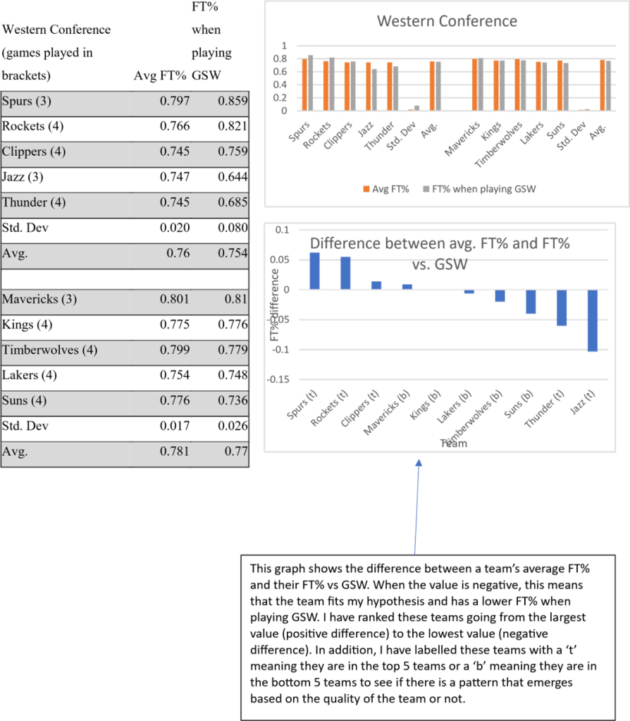
Below is the data that I have collected from the 2016-17 NBA season. For the purpose of consistency,
I have removed any playoff (post-season) games from the data. In order to test the effect across both
good and bad teams, I have taken the FT% from the top 5 teams and bottom 5 teams from each
conference to compare. Due to the fact that the Golden State Warriors (GSW) were the first team in
the Western Conference in the 2016-17 season, I have taken the 5 teams that come after them i.e
teams 2-6 rather than 1-5. As for the 2017-18 season where GSW finished second in the Western
Conference, I have taken teams 1,3,4,5,6. This is done to maintain sample sizes across both
conferences. I have taken the average FT% as a decimal where 1 would be all free throws that are
attempted are made and 0 would be when all free throws attempted are missed. In addition, I have
compiled the data into 2 bar charts to compare the conferences. Furthermore, I have taken the average
of the teams’ average FT% and then also the average of their average FT% when playing GSW.

2017-18

Avg FT%

Western Conference when (games played in playing brackets) Avg FT% GSW

Rockets (3)		0.781	0.655
Trail Blazers (3)		0.8	0.858
Thunder (3)		0.716	0.707
Jazz (3)		0.779	0.742
Pelicans (4)		0.772	0.676
Std. Dev		0.028	0.072
Avg		0.77	0.728
Lakers (4)		0.714	0.689
Kings (4)		0.735	0.756
Mavericks (4)		0.763	0.713
Grizzlies (3)		0.786	0.769
Suns (4)		0.741	0.738
Std. Dev		0.025	0.029
Avg		0.748	0.733

Avg FT%

Eastern Conference when (games played in playing brackets) Avg FT% GSW

Raptors (2)		0.794	0.896
Celtics (2)		0.771	0.788
76ers (2)		0.752	0.725
Cavaliers (2)		0.779	0.761
Pacers (2)		0.779	0.7
Std. Dev		0.014	0.068
Avg		0.775	0.774

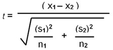
To recall, my hypothesis was that the average FT% when playing GSW would be lower than teams’ average FT% across the whole season. So, keeping this in mind, we can look at the data to test this.

Taking the top 5 teams in the Western Conference, the average FT% for the teams in this data set was 0.76. In the same data set, when playing GSW their average FT% was 0.754. This represents a 0.6% decrease in FT% when playing a superstar team. Moving on to the bottom 5 teams in the Western Conference, their average FT% across the season was 0.781. However, when playing GSW, their FT% was 0.77. This represents a 1.1% decrease. This is particularly interesting as in Jennifer Brown’s research, she found that when the opposition to a superstar is of a higher quality, their decrease in performance is greater than that of an opposition with a lower quality. However, in the Western Conference data that I have collected, the impact of a superstar team seems to be the opposite to this as lower quality teams deviate more from their average FT% when playing a superstar team than higher quality oppositions. Moving on to the Eastern Conference, the top 5 teams’ average FT% was 0.773 but when playing GSW, their FT% was 0.774. This represents a 0.01% increase in FT%, going against my hypothesis. Looking at the bottom 5 teams, their average FT% was 0.782, but when playing GSW their FT% was only 0.726. This represents a 5.6% decrease when playing a superstar team. This, again, goes against Jennifer Brown’s findings in that once again the lower quality teams deviate more from their average when playing GSW. Moreover, looking at the standard deviation in the Western Conference, there appears to be more inconsistency in the top 5 teams compared to the bottom 5 teams. However, across both sets the standard deviation is higher when playing GSW than the season average. This shows the superstar effect as when playing against a superstar team, players’ confidence might be low and stress levels may be high leading to higher inconsistency in their performance. This pattern is seen in the Eastern Conference as well as the standard deviation when playing GSW is higher in both data sets implying higher inconsistency when playing against a superstar team. However, in the Eastern Conference, this inconsistency is higher when looking at the bottom 5 teams compared to the top 5 teams. 

Analysis (2017-18):

The Golden State Warriors’ core lineup had stayed the same throughout the 2017-18 season as well as there were still 4 All-Stars on their starting lineup. So I was able to gather data from this year as well to try and bolster my data. When analysing the Western Conference, the pattern remains the same as the average FT% when playing against the GSW is lower for both the top 5 teams as well as the bottom 5 teams. However, there is less of a correlation when looking at the Eastern Conference. In fact, in the top 5 teams, the average FT% only decreases by 0.1% and in the bottom 5 teams, the average FT% actually increases by 0.6%. This increase may be attributed to the lack of games played between GSW and Eastern Conference teams. Information on this may be found in the appendix as to how the number of games that GSW plays against each time is decided. The standard deviation fits with the pattern seen in the 2016-17 season in that on all accounts, the standard deviation is higher when teams play against a superstar team, once again implying higher inconsistency due to the superstar effect. 

T-test:

Above is the general formula for the t-test. This is a significance test that helps me to clarify whether my data suggests a correlation or not. I have laid out the maths working in Appendix 2 where I have shown what my null and alternative hypothesis as well as which letters in the formula correspond to which values in my data. As seen in Appendix 2, the p-value that I obtained is 0.004 to three significant figures. When testing to a 1% significance level, this p-value suggests a correlation as it is smaller than 0.01. This essentially means that there is less than a 1% chance that the correlation that my data presents is up to chance. Meaning that there is a 99% chance that it is due to some other factor. In these circumstances it is safe to assume that this other factor is the superstar effect as this is the only change in the two data sets (whether or not a team plays GSW).  

Conclusion:

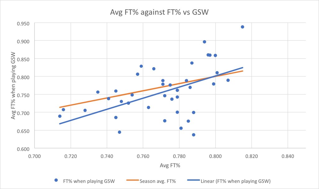
Above is a scatter plot of every single data point I had available to me. This shows the teams’ average FT% on the x-axis and the teams’ FT% when playing GSW on the y-axis. The orange line represents a theoretical line of best fit showing a situation where the FT% would not change regardless of whether a team plays GSW or not. The blue line shows the actual line of best fit of my data. As seen on the graph, the blue line is significantly below the orange line when a team’s season average FT% is low. Then as you progress across the x-axis, the gap between the two lines gradually closes and actually the blue line is above the orange line at the end. This suggests two things: one is that when a team’s average FT% is already low, they play relatively much worse against GSW than a team whose season average FT% is higher. The second thing is that after a certain point on the x-axis (approx. 80% average FT%), a team generally plays better against GSW than they do against other teams. When taking the data as a whole, using the t-test I can reject the null hypothesis but this section when a team plays better than average against the superstar team suggests otherwise. Furthermore, a higher average FT% doesn’t always suggest a ‘better’ team (top 5 in their conference) and vice versa. Generally, in basketball, a team’s free throw percentage is actually a fairly insignificant factor in actually winning a game. Teams that finish at the top of their conferences do so because they shoot more efficiently in open play or defend better as a team rather than by shooting a higher free throw percentage than the other team. In fact, theoretically, every team should shoot the same free throw percentage as they are supposedly all in the same situation – they all shoot from the same distance from the basket. The factors that influence FT% are more than the quality of the team (e.g influence of home crowd, high pressure situations (clutch moments), style of play (some teams play to get to the free throw line more often)). Potentially, teams with an already high FT% may recognise this strength and they can use this to try and beat GSW (even if it is only a small part of the game) and so they shoot higher than average against GSW. However this is only speculation and would need further research to justify this claim. 

 I also wanted to test the superstar effect depending on the quality of the opposition to the GSW. As you may recall, in Jennifer Brown’s study, she found that generally the superstar effect was more pronounced when the opposition was of higher quality (explained in introduction). So I wanted to test this finding with my data.  To see this, I took the average FT% of all of the ‘worst’ teams (bottom 5 teams) and the average FT% of the ‘best’ teams (top 5 teams). Then I took the average FT% when playing GSW of these two data sets to compare them. When looking at the top 5 teams, I saw a 1.2% decrease in FT% when playing GSW and when looking at the bottom 5 teams, there was a 1.9% decrease in FT%. While both percentages decreased, it is interesting to see that when GSW played lower quality teams, their FT% decreased more than that of higher quality teams. While I can only hypothesise why this may be, this may be down to numerous factors. For example, lower quality teams often have young, inexperienced players who may not be able to handle the pressure of playing against a superstar team. This may be caused by roster instability which is commonly found in lower quality teams. These teams often change around their players meaning fewer players experience consistent game time. So their ability to handle pressure is reduced. This idea is specific to team sports and may be why my data contradicts Brown’s findings. However, again, this is only a hypothesis and would need further research and data to support it.  

Lastly, there are other outcomes caused by the superstar effect in the NBA. Teams that play superstars often receive higher revenues from ticket sales due to the popularity generated from the players. For example, a study conducted by Jerry Hausman and Gregory Leonard showed that Michael Jordan was worth approximately $50 million to other teams (Hausman, J. Leonard, G. 1997). This may be due to the fact that Jordan, being a superstar, increases attendance at away games creating an extra 5,631 fans on average (Humphreys Brad.R and Johnson, C, 2017). This is quite interesting as even though a team may play worse due to the superstar effect, that same effect can actually benefit the team financially. This money could then be used to try and buy new, better players or higher quality coaches and practice facilities to make the team more competitive.

Appendix 1:

In this section, I will explain how the NBA works for those that are not familiar with the sport/league.

The NBA stands for the National Basketball Association and is played in the USA and Canada (Toronto). The league consists of 30 teams, 15 of which are part of the Eastern Conference and the other 15 in the Western Conference. Teams located on the east coast are part of the Eastern Conference and teams located on the west coast of the country are part of the Western Conference.

Every year, there is a regular season where 1,230 games take place and each team plays 82 games. After the regular season, there is a playoff tournament in a knock-out format where the top 8 teams of each conference are selected to be part of the playoffs. However this is not relevant to my data as I am only analysing the regular season and so I will not explain how the playoff tournament works exactly. As part of the 82 regular season games that each team plays, 30 of these are from playing against teams from the other conference. Each team will play every team from the other conference twice totalling to 30 games. In addition they will play teams in their division 4 times every year, totalling to 16 games as there are 5 teams in each division so any given team will play the other 4 teams in their division 4 times each. There are 6 divisions in the league and each one contains teams only from one conference. So this leaves 36 games to be played against the other 10 teams in a given team’s conference. So a team would play the other 10 teams either 3 or 4 times in a year. This varies year on year.  All of this totals to 82 games. 

Appendix 2:

In this section, you will find extra maths working related to the t-test that is discussed earlier in the paper. 

T = 

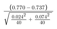
Above is the t-test formula when the numbers I am using have been inputted. I am using a two-sample test as I am comparing two different data sets. In addition, I will be using a one-tailed test as I am testing whether the average of one data set is lower than the other rather than just different to the other data set. This significance test will help me to see if my data has a significant correlation and will help me to decide which hypothesis to accept/reject. In this situation, my null hypothesis is that the average FT% when playing GSW would not change compared to a team’s season average. My alternative hypothesis is that the FT% of a team when playing against the GSW would be lower than their season average. In order to try and maximise my sample size, I will be taking the average FT% of all teams recorded across both seasons. This makes my total sample size (n) as 80. This also means that my degrees of freedom is 78 (n-2). I will take the teams’ average FT% across the season as X₁ and the average when playing GSW as X₂. S₁ will represent the standard deviation for the season average FT% and S₂ will represent the standard deviation for the average FT% when playing GSW. N₁ and N₂ will be the same value (40) as the size of the data sets are the same. So when putting all the numbers in the formula, the t-value that is obtained is 2.68 to 3 significant figures. When using an online t-test calculator (https://www.omnicalculator.com/statistics/t–test), the p-value obtained is 0.00448917.

References:

Brown, J. (2011). Quitters Never Win: The (Adverse) Incentive Effects of Competing with

Superstars. Journal of Political Economy, 119(5), 982–1013. https://doi.org/10.1086/663306

Rosen, S. (1981). The Economics of Superstars. The American Economic Review, 71(5), 845–858.

http://www.jstor.org/stable/1803469

Hausman, J. A., & Leonard, G. K. (1997). Superstars in the National Basketball Association:

Economic Value and Policy. Journal of Labor Economics, 15(4), 586–624.

https://doi.org/10.1086/209839

Humphreys, Brad R. and Johnson, Candon, The Effect of Superstar Players on Game Attendance:

Evidence from the NBA (July 31, 2017). Available at

SSRN: https://ssrn.com/abstract=3004137 or http://dx.doi.org/10.2139/ssrn.3004137

LandOfBasketball.com, Information About NBA Players, Teams and Championships. (no date). Available at: https://www.landofbasketball.com/.

Basketball Statistics & History of Every Team & NBA and WNBA Players | Basketball Reference.com (no date). Available at: https://www.basketball–reference.com/.